7. A closer look at Lie groups (continued)
Conjugation and the adjoint
In the first part, we defined how a group acts on a set. A group can also act on itself: from the left, from the right, or by conjugation. For \(g, h_1, h_2 \in \mathrm{G}\), we say that \(h_2\) is the conjugate of \(h_1\) by \(g\) if
\[h_2 = g h_1 g^{-1}.\]The map \(h \mapsto g h g^{-1}\) is the conjugation map of the group. Note that \(g h g^{-1} \in \mathrm{G}\), because the group is closed under its operator.
The group also acts on its Lie algebra by conjugation; this action is the adjoint. Formally, the adjoint is the derivative of conjugation at the identity. Let \(\gamma(t)\) be a path in the group with \(\gamma(0) = e\) and \(\dot\gamma(0) = \rho^\wedge \in \mathfrak{g}\). Then
\[\left. \frac{\mathrm{d}}{\mathrm{d}t} \big( g \gamma(t) g^{-1} \big) \right|_{t = 0} = g \rho^\wedge g^{-1},\]and we define the adjoint of \(g\) as
\[\mathrm{Ad}_g : \mathfrak{g} \to \mathfrak{g}, \qquad \rho^\wedge \mapsto \mu^\wedge = g \rho^\wedge g^{-1}. \tag{14}\]So the adjoint is conjugation by the group, applied to the Lie algebra. It maps an element of \(\mathfrak{g}\) to another element of \(\mathfrak{g}\); notice that (14) is exactly the expression (5) we met in the previous part. Some references, such as Solà et al., describe the adjoint as a map from the tangent space at \(g\) to the Lie algebra. The two views are related through (2), and the last section of this part shows how the adjoint, the tangent space at \(g\) and the Lie algebra fit together.
The adjoint has two properties. For \(g, g_1, g_2 \in \mathrm{G}\), \(\rho^\wedge, u^\wedge \in \mathfrak{g}\) and scalars \(a, b\):
- Linearity: \(\mathrm{Ad}_g(a \rho^\wedge + b u^\wedge) = a\, \mathrm{Ad}_g(\rho^\wedge) + b\, \mathrm{Ad}_g(u^\wedge)\).
- Composition: \(\mathrm{Ad}_{g_1}\big(\mathrm{Ad}_{g_2}(\rho^\wedge)\big) = \mathrm{Ad}_{g_1 g_2}(\rho^\wedge)\).
With the adjoint, the last property of the exponential map from the previous part can be written in three equivalent ways:
\[\exp\big(\mathrm{Ad}_g(\rho^\wedge)\big) = g \exp(\rho^\wedge) g^{-1} \iff \exp\big(\mathrm{Ad}_g(\rho^\wedge)\big)\, g = g \exp(\rho^\wedge) \iff g^{-1} \exp\big(\mathrm{Ad}_g(\rho^\wedge)\big) = \exp(\rho^\wedge)\, g^{-1}.\]The adjoint matrix
Since the adjoint is linear, there is a matrix that maps \(\rho \in \mathbb{R}^n\) directly to \(\mu \in \mathbb{R}^n\). We call it the adjoint matrix and denote it by \(T\). Applying \(\vee\) to (14) gives
\[T \rho = \mu = \big( g \rho^\wedge g^{-1} \big)^\vee. \tag{15}\]To find \(T\), we compute the right-hand side of (15) and write it in the form of the left-hand side. Here are two examples.
\(\mathrm{SO}(3)\). From the previous part, \(\rho = \omega^b\) and \(\mu = \omega^s\), and \(\omega^s = R \omega^b\), so \(T_R = R\). Using (15) and (8) gives the same answer:
\[\mu = \big( R\, \omega^{b\wedge} R^\top \big)^\vee = \big( (R \omega^b)^\wedge \big)^\vee = R \omega^b.\]\(\mathrm{SE}(3)\). From the previous part, \(\rho = \begin{bmatrix} \omega^b \\ v^b \end{bmatrix}\) and \(\mu = \begin{bmatrix} \omega^s \\ v^s \end{bmatrix}\). Using the kinematics (12),
\[\mu = \begin{bmatrix} \omega^s \\ v^s \end{bmatrix} = \underbrace{\begin{bmatrix} R & 0 \\ [p]_\times R & R \end{bmatrix}}_{T_{R,p}} \underbrace{\begin{bmatrix} \omega^b \\ v^b \end{bmatrix}}_{\rho}. \tag{16}\]Let us check this with (15). For \(\mathrm{SE}(3)\),
\[g = \begin{bmatrix} R & p \\ 0 & 1 \end{bmatrix}, \qquad g^{-1} = \begin{bmatrix} R^\top & -R^\top p \\ 0 & 1 \end{bmatrix}, \qquad \rho^\wedge = \begin{bmatrix} [\omega^b]_\times & v^b \\ 0 & 0 \end{bmatrix},\]so
\[\begin{aligned} \mu &= \left( \begin{bmatrix} R & p \\ 0 & 1 \end{bmatrix} \begin{bmatrix} [\omega^b]_\times & v^b \\ 0 & 0 \end{bmatrix} \begin{bmatrix} R^\top & -R^\top p \\ 0 & 1 \end{bmatrix} \right)^\vee = \begin{bmatrix} [R \omega^b]_\times & -[R \omega^b]_\times p + R v^b \\ 0 & 0 \end{bmatrix}^\vee \\ &= \begin{bmatrix} [R \omega^b]_\times & [p]_\times R \omega^b + R v^b \\ 0 & 0 \end{bmatrix}^\vee = \begin{bmatrix} R \omega^b \\ [p]_\times R \omega^b + R v^b \end{bmatrix} = \underbrace{\begin{bmatrix} R & 0 \\ [p]_\times R & R \end{bmatrix}}_{T_{R,p}} \underbrace{\begin{bmatrix} \omega^b \\ v^b \end{bmatrix}}_{\rho}, \end{aligned}\]the same as (16).
The Lie bracket
There are two ways to define the Lie bracket: through its relation to the adjoint, and through the definition of an algebra. We briefly discuss both.
The adjoint is the action of the group on its Lie algebra, the derivative of conjugation at the identity. The Lie bracket is, in a sense, the action of the Lie algebra on itself, with no group element involved. To derive it, we differentiate the adjoint once more, now with respect to the group element: let \(g = \gamma(t)\) be a path with \(\gamma(0) = e\) and \(\dot\gamma(0) = \tau^\wedge \in \mathfrak{g}\). Using \(\frac{\mathrm{d}}{\mathrm{d}t} \gamma^{-1} = -\gamma^{-1} \dot\gamma \gamma^{-1}\),
\[\frac{\mathrm{d}}{\mathrm{d}t} \mathrm{Ad}_{\gamma(t)}(\rho^\wedge) = \frac{\mathrm{d}}{\mathrm{d}t} \big( \gamma \rho^\wedge \gamma^{-1} \big) = \dot\gamma \rho^\wedge \gamma^{-1} - \gamma \rho^\wedge \gamma^{-1} \dot\gamma \gamma^{-1},\]and at \(t = 0\), where \(\gamma(0) = e\),
\[\left. \frac{\mathrm{d}}{\mathrm{d}t} \mathrm{Ad}_{\gamma(t)}(\rho^\wedge) \right|_{t = 0} = \tau^\wedge \rho^\wedge - \rho^\wedge \tau^\wedge.\]This leads to the definition of the Lie bracket of two elements \(X, Y \in \mathfrak{g}\):
\[[X, Y] = XY - YX.\]The second way comes from the definition of an algebra. An algebra is a vector space equipped with a bilinear product. For a Lie algebra, this product is the Lie bracket \([\cdot, \cdot] : \mathfrak{g} \times \mathfrak{g} \to \mathfrak{g}\), which is antisymmetric, \([X, Y] = -[Y, X]\), and satisfies the Jacobi identity
\[[X, [Y, Z]] + [Y, [Z, X]] + [Z, [X, Y]] = 0 \qquad \text{for all } X, Y, Z \in \mathfrak{g}.\]For \(\mathrm{SO}(3)\), the Lie bracket is the cross product in disguise: \([\omega_1^\wedge, \omega_2^\wedge] = (\omega_1 \times \omega_2)^\wedge\). For the generators of \(\mathfrak{so}(3)\) from the previous part, for example, \([E_1, E_2] = -[E_2, E_1] = E_3\), just as \(e_1 \times e_2 = e_3\).
The adjoint, tangent spaces and coordinate frames
Finally, let us see how the adjoint relates to the map between a tangent space and the Lie algebra, and to the body and spatial (world) frames we use in robotics.
First, note that tangent spaces correspond to velocities, but any vector can be mapped to them, not only velocities. A good example is a noise vector in a filter: on \(\mathrm{SE}(3)\), a noise vector \(n \in \mathbb{R}^6\) can be mapped to the Lie algebra with the wedge operator, even though it is not a velocity.
Now consider a robot moving in \(\mathrm{SE}(3)\), currently at \(g = \begin{bmatrix} R & p \\ 0 & 1 \end{bmatrix}\). We measure its velocities in the body frame, \(\rho = \begin{bmatrix} \omega^b \\ v^b \end{bmatrix}\). Like any other vector, \(\rho\) can be mapped to \(\mathfrak{se}(3)\),
\[\rho^\wedge = \begin{bmatrix} \omega^b \\ v^b \end{bmatrix}^\wedge = \begin{bmatrix} [\omega^b]_\times & v^b \\ 0 & 0 \end{bmatrix},\]and also to the tangent space \(T_g \mathrm{SE}(3)\), using (3) and (4):
\[{}^{g}\!\rho^\wedge = g \rho^\wedge = \begin{bmatrix} R & p \\ 0 & 1 \end{bmatrix} \begin{bmatrix} [\omega^b]_\times & v^b \\ 0 & 0 \end{bmatrix}.\]If we now multiply \({}^{g}\!\rho^\wedge\) by \(g^{-1}\) on the right, we map it back to \(\mathfrak{se}(3)\), but we do not recover \(\rho^\wedge\). We get a new element of the Lie algebra; call it \(\mu^\wedge\):
\[\mu^\wedge = {}^{g}\!\rho^\wedge\, g^{-1} = \begin{bmatrix} R & p \\ 0 & 1 \end{bmatrix} \begin{bmatrix} [\omega^b]_\times & v^b \\ 0 & 0 \end{bmatrix} \begin{bmatrix} R^\top & -R^\top p \\ 0 & 1 \end{bmatrix}.\]As we saw in the previous part, this \(\mu^\wedge\) is \(\begin{bmatrix} \omega^s \\ v^s \end{bmatrix}^\wedge\): the same velocities, expressed in the spatial frame, mapped to \(\mathfrak{se}(3)\). This is the adjoint. So, in the context of \(\mathrm{SE}(3)\), the adjoint takes the body-frame velocities mapped to \(\mathfrak{se}(3)\), carries them to \(T_g \mathrm{SE}(3)\) by left multiplication with \(g\), and brings them back to \(\mathfrak{se}(3)\) by right multiplication with \(g^{-1}\), which gives the spatial-frame velocities. This is shown in the figure below.
One might think that, because \(\rho\) holds the velocities of the body at \(g\), it represents \(T_g \mathrm{SE}(3)\), so \(\rho^\wedge\) should live in \(T_g \mathrm{SE}(3)\). This is not true: the wedge operator (4) maps any vector to \(\mathfrak{se}(3)\), even a vector of velocities at \(g\).
Another source of confusion is the difference between transforming between two coordinate frames and transforming between two tangent spaces. Consider a vector \(x^b\) expressed in the body frame (the frame at \(g\)), and the same vector \(x^s\) expressed in the spatial frame (the frame at the identity). The element of \(\mathfrak{g}\) that corresponds to \({}^{g}x^{b\wedge} \in T_g \mathrm{G}\) is not \(x^{s\wedge}\); by (2), it is simply \(g^{-1}\, {}^{g}x^{b\wedge} = x^{b\wedge}\). To get \(x^{s\wedge}\), we have to multiply by \(g^{-1}\) on the right instead:
\[x^{s\wedge} = {}^{g}x^{b\wedge}\, g^{-1} = g\, x^{b\wedge} g^{-1} = \mathrm{Ad}_g\big(x^{b\wedge}\big).\]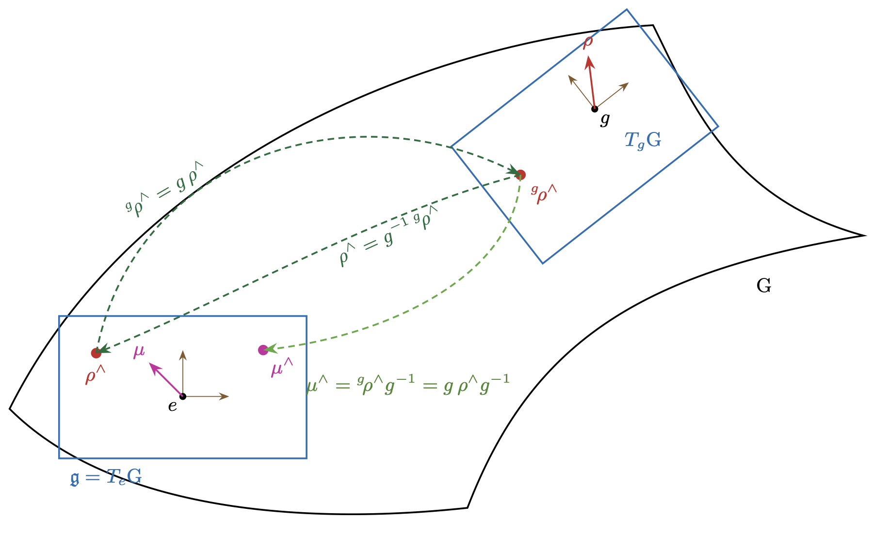
Further reading
- M. Ghaffari, ROB 530: Mobile Robotics, University of Michigan: lecture notes with a complete treatment of matrix Lie groups for robotics.
- J. Solà, J. Deray, and D. Atchuthan, A micro Lie theory for state estimation in robotics, arXiv:1812.01537, 2018: also covers the plus and minus operators, Jacobians and derivatives on Lie groups.
- F. C. Park, The Optimal Kinematic Design of Mechanisms, Ph.D. thesis, Harvard University, 1991: a detailed treatment of Jacobians on Lie groups.